A SerDes system transmitter can often be modeled with a feed-forward equalizer (FFE) and low pass filter (LPF).
Our Model Generation Tool for a Tx IBIS-AMI model with an FFE and LPF can be used to specify the requirements for this Tx model with intended use in a Channel Simulator that conforms with the IBIS-AMI standard.
For a general aid to understanding an FFE see our FFE Analysis Tool.
A Tx IBIS-AMI model with an FFE and LPF can be specified by listing various requirements in four specific steps.
- General information: For the model name and intended usage for bit rate
- IBIS data: For the model IBIS analog out buffer characteristics.
- Jitter data. For the model data jitter characteristics.
- FFE + LPF data. For the model FFE and LPF characteristics.
- Complete and send us your model specification.
Each of these model specification steps are discussed here in detail. Go back to the prior page to start entering your model specification data. Go back...
1. General information for a Tx IBIS-AMI model
It is convenient to start by giving a name to your model. Often this can be a composite string composed of your company name and the associated Tx HSD IC part or application.
For example, a typical model name has this construction:
<my_company>_<part_number>_<application>
such as:
HSD_A2357_PCIe3
The nominal bit rate should also be listed, though the model will automatically adjust itself for other bit rates.
For example, for PCIe3, the nominal bit rate is 8 Gbps.
2. IBIS data for a Tx IBIS-AMI model
A Tx HSD IC often has its output buffer modeled based on the industry IBIS standard.
Since our Tx model is intended for use in a Channel Simulator, only a subset of the IBIS standard is applicable. A Channel Simulator is defined for achieving fast simulation speed for millions or more bits compared to industry standard SPICE based circuit transient simulation.
Based on industry conventions, a Channel Simulator will only use linear characteristics from a defined IBIS buffer. If the IBIS buffer model contains any nonlinearities, then the Channel Simulator will determine the best fit for linear characteristic to be used with the Channel Simulation. If any actual nonlinearities are intended to be associated with the Tx model then they should be defined in the AMI portion of an IBIS-AMI model and not in the IBIS portion.
In general, the Tx output IBIS buffer for use with a Channel Simulator has this schematic view:
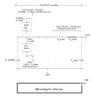
This schematic is a representation for a Tx HSD IC output buffer that has differential output pins intended for use with a differential channel.
The IBIS standard defines these specific characteristics.
C_pkg: default packaging capacitance of the component pins.
L_pkg: default packaging inductance of the component pins.
R_pkg: default packaging resistance of the component pins.
C_comp: defines die capacitance and should not include the capacitance of the package.
Pullup: defines the I-V tables of the pullup structures of an output buffer.
Pulldown: defines the I-V tables of the pulldown structures of an output buffer.
Rise time (dV/dt_r): defines the rise time of a buffer. The ramp rate does not include packaging but does include the effects of the C_comp parameter.
Fall time (dV/dt_f): defines the rise time of a buffer. The ramp rate does not include packaging but does include the effects of the C_comp parameter.
The rise and fall time is defined as the time it takes the output to go from 20% to 80% of its final value. The ramp rate is defined as:
![]()
The ramp rate must be specified as an explicit fraction and must not be reduced.
For example: 1.0 / 1e-12
For the above parameters, the IBIS buffer specification includes the ability to list their typical, minimum and maximum values.
3. Jitter data for a Tx IBIS-AMI model
A Tx HSD IC often adds jitter to its input data. Jitter can be have many different characteristics.
One view of the different constituent components to total jitter is seen in this classification of jitter types.

Based on the industry IBIS-AMI standard, a Tx model can have these associated jitter characteristics:
Time(n) is the time of the nth clock modified when creating input waveforms for the Tx.
Random (Tx_Rj): Definition: The standard deviation of a white Gaussian phase noise process at the transmitter which is to be added to the behavior implemented by the EDA tool by modifying the stimulus input or by post processing the simulation results. Entries are assumed to be in units of seconds when declared as Type Float.
Time(n) = n * bit_time + Tx_Rj * gaussian_rand()
Where gaussian_rand() is a function that returns floating point numbers between -inf and +inf. The distribution of these numbers shall be a white Gaussian distribution centered at 0.0 with a standard deviation of 1.0. The EDA tool can protect against abs(Tx_Rj*gaussian_rand()) > 0.5UI.
Deterministic (Tx_Dj): Definition: The worst case half the peak to peak variation at the transmitter implemented by the EDA tool by modifying the stimulus input or by post processing the simulation results. Tx_Dj shall include all deterministic and uncorrelated bounded jitter that is not accounted for by Tx_DCD, and Tx_Sj. Entries are assumed to be in units of seconds when declared as Type Float.
Time(n) = n * bit_time + 2.0 * Tx_Dj * rand()
Where rand() is a function that returns floating point numbers between -0.5 and +0.5 with white uniform distribution.
Duty Cycle Distortion (Tx_DCD): Definition: Tx_DCD (Transmit Duty Cycle Distortion) defines half the peak to peak clock duty cycle distortion to be added to the behavior implemented by the EDA tool by modifying the stimulus input or by post processing the simulation.
Time(n) = n * bit_time + Tx_DCD * (-1.0)^n
Periodic (Tx_Sj, Tx_Sj_Frequency):
Time(n) = n * bit_time + Tx_Sj * sin( n * bit_time * 2.0 * Pi * Tx_Sj_Frequency)
Tx_Sj Definition: Half the peak to peak amplitude of a sinusoidal jitter which is to be added to the behavior implemented directly by the transmitter model.
Usage Rules: If Tx_Sj_Frequency is not assigned (either in the model or by the user), Tx_Sj should be ignored. Entries are assumed to be in units of seconds when declared as Type Float.
Tx_Sj_Frequency Definition: The frequency, in hertz, of the sinusoidal jitter at the transmitter.
Usage Rules: If Tx_Sj_Frequency is not assigned (either in the model or by the user), Tx_Sj should be ignored.
The total jitter usable with a Channel Simulation should be less than 1/2 UI where UI = 1/(data bit time) in seconds. Since Rj is unbounded, the Channel Simulator limits Rj to 1/2 UI.
4. FFE and LPF data for a Tx IBIS-AMI model
For a general aid to understanding an FFE see our FFE Analysis Tool.
Here, the discussion is focused on the FFE and LPF data to be entered for the Tx IBIS-AMI model.
Data can be entered for the FFE and the LPF. For most data, one can enter data for typical, slow and fast process corners. The actual use of <typ>, <slow>, <fast> is carried out by the EDA tool based on its Channel Simulator corner setting.
For the FFE, data is entered for the pre-cursor and post-cursor values. For example, values for PreCursor1TypDefault, PostCursor1TypDefault, and PostCursor2TypDefault. One can define as many pre-cursors and post-cursors as desired. For each pre-cursor and post-cursor, one enters the default value and a list of values for each process corner. The lists define allowed values. For example, values for PreCursors1Typ, PostCursors1Typ, and PostCursors2Typ are list parameter. The default value is used for the Channel Simulation.
For the FFE using the pre- and post-cursor default values, the FFE response can be normalized based on the setting for CursorNormalization. See Typical FFE Characteristics and Displays… for discussion of the CursorNormalization options.
For the FFE, one has the option of allowing the model to automatically set the pre-cursor and post-cursor values (and ignore the default value settings) to equalize the channel being used with this Tx model. This option is enabled by setting AdaptFFE=1. When enabled, one can further specify whether the combined FFE+LPF+Channel response should be normalized for unity frequency domain response at 0 Hz (AdaptChLoss=1) or for unity frequency domain response at the Nyquist frequency (AdaptChLoss=2). Additionally, one can further specify whether the channel equalized FFE values should be forced to the nearest values in the pre- and post-cursor lists (AdaptToList=1).
For the LPF, data is entered for the frequency domain poles in Hz. All poles are entered as positive frequency values. One can define as many poles as desired. However, only those poles less than half of the simulation sample rate are used for simulation.
5. Complete and send us your model specification
When one is satisfied with the model specification data entered, then the model requirements can be sent to SerDesDesign.com for an estimate on the consulting fee for creating the custom IBIS-AMI model by selecting the Send button on the prior page.
Go back to the prior page to complete entering your model specification data. Go back…